# Copyright 2025 Google LLC
#
# Licensed under the Apache License, Version 2.0 (the "License");
# you may not use this file except in compliance with the License.
# You may obtain a copy of the License at
#
#     https://www.apache.org/licenses/LICENSE-2.0
#
# Unless required by applicable law or agreed to in writing, software
# distributed under the License is distributed on an "AS IS" BASIS,
# WITHOUT WARRANTIES OR CONDITIONS OF ANY KIND, either express or implied.
# See the License for the specific language governing permissions and
# limitations under the License.
BigFrames Timedelta#
|
|
|
|
In this notebook, you will use timedeltas to analyze the taxi trips in NYC.
Setup#
import bigframes.pandas as bpd

PROJECT = "bigframes-dev" # replace this with your project
LOCATION = "us" # replace this with your location

bpd.options.bigquery.project = PROJECT
bpd.options.bigquery.location = LOCATION
bpd.options.display.progress_bar = None

bpd.options.bigquery.ordering_mode = "partial"
Timedelta arithmetics and comparisons#
First, you load the taxi data from the BigQuery public dataset bigquery-public-data.new_york_taxi_trips.tlc_yellow_trips_2021. The size of this table is about 6.3 GB.
taxi_trips = bpd.read_gbq("bigquery-public-data.new_york_taxi_trips.tlc_yellow_trips_2021").dropna()
taxi_trips = taxi_trips[taxi_trips['pickup_datetime'].dt.year == 2021]
taxi_trips.peek(5)
| vendor_id | pickup_datetime | dropoff_datetime | passenger_count | trip_distance | rate_code | store_and_fwd_flag | payment_type | fare_amount | extra | mta_tax | tip_amount | tolls_amount | imp_surcharge | airport_fee | total_amount | pickup_location_id | dropoff_location_id | data_file_year | data_file_month | |
|---|---|---|---|---|---|---|---|---|---|---|---|---|---|---|---|---|---|---|---|---|
| 0 | 1 | 2021-06-09 07:44:46+00:00 | 2021-06-09 07:45:24+00:00 | 1 | 2.200000000 | 1.0 | N | 4 | 0E-9 | 0E-9 | 0E-9 | 0E-9 | 0E-9 | 0E-9 | 0E-9 | 0E-9 | 263 | 263 | 2021 | 6 |
| 1 | 2 | 2021-06-07 11:59:46+00:00 | 2021-06-07 12:00:00+00:00 | 2 | 0.010000000 | 3.0 | N | 2 | 0E-9 | 0E-9 | 0E-9 | 0E-9 | 0E-9 | 0E-9 | 0E-9 | 0E-9 | 263 | 263 | 2021 | 6 |
| 2 | 2 | 2021-06-23 15:03:58+00:00 | 2021-06-23 15:04:34+00:00 | 1 | 0E-9 | 1.0 | N | 1 | 0E-9 | 0E-9 | 0E-9 | 0E-9 | 0E-9 | 0E-9 | 0E-9 | 0E-9 | 193 | 193 | 2021 | 6 |
| 3 | 1 | 2021-06-12 14:26:55+00:00 | 2021-06-12 14:27:08+00:00 | 0 | 1.000000000 | 1.0 | N | 3 | 0E-9 | 0E-9 | 0E-9 | 0E-9 | 0E-9 | 0E-9 | 0E-9 | 0E-9 | 143 | 143 | 2021 | 6 |
| 4 | 2 | 2021-06-15 08:39:01+00:00 | 2021-06-15 08:40:36+00:00 | 1 | 0E-9 | 1.0 | N | 1 | 0E-9 | 0E-9 | 0E-9 | 0E-9 | 0E-9 | 0E-9 | 0E-9 | 0E-9 | 193 | 193 | 2021 | 6 |
Based on the dataframe content, you calculate the trip durations and store them under the column “trip_duration”. You can see that the values under “trip_duartion” are timedeltas.
taxi_trips['trip_duration'] = taxi_trips['dropoff_datetime'] - taxi_trips['pickup_datetime']
taxi_trips['trip_duration'].dtype
duration[us][pyarrow]
To remove data outliers, you filter the taxi_trips to keep only the trips that were less than 2 hours.
import pandas as pd

taxi_trips = taxi_trips[taxi_trips['trip_duration'] <= pd.Timedelta("2h")]
Finally, you calculate the average speed of each trip, and find the median speed of all trips.
average_speed = taxi_trips["trip_distance"] / (taxi_trips['trip_duration'] / pd.Timedelta("1h"))
print(f"The median speed of an average taxi trip is: {average_speed.median():.2f} mph.")
The median speed of an average taxi trip is: 10.58 mph.
Given how packed NYC is, a median taxi speed of 10.58 mph totally makes sense.
Use timedelta for rolling aggregation#
Using your existing dataset, you can now calculate the taxi trip count over a period of two days, and find out when NYC is at its busiest and when it is fast asleep.
First, you pick two workdays (a Thursday and a Friday) as your target dates:
import datetime

target_dates = [
    datetime.date(2021, 12, 2),
    datetime.date(2021, 12, 3)
]

two_day_taxi_trips = taxi_trips[taxi_trips['pickup_datetime'].dt.date.isin(target_dates)]
print(f"Number of records: {len(two_day_taxi_trips)}")
# Number of records: 255434
Number of records: 255434
Your next step involves aggregating the number of records associated with each unique “pickup_datetime” value. Additionally, the data undergo upsampling to account for any absent timestamps, which are populated with a count of 0.
import pandas as pd

two_day_trip_count = two_day_taxi_trips['pickup_datetime'].value_counts()

full_index = pd.date_range(
    start='2021-12-02 00:00:00',
    end='2021-12-04 00:00:00',
    freq='s',
    tz='UTC'
)
two_day_trip_count = two_day_trip_count.reindex(full_index).fillna(0)
You’ll then calculate the sum of trip counts within a 5-minute rolling window. This involves using the rolling() method, which can accept a time window in the form of either a string or a timedelta object.
two_day_trip_rolling_count = two_day_trip_count.sort_index().rolling(window="5m").sum()
Finally, you visualize the trip counts throughout the target dates.
from matplotlib import pyplot as plt
import matplotlib.dates as mdates

plt.figure(figsize=(16,7))
ax = plt.gca()
formatter = mdates.DateFormatter("%D %H:%M:%S")
ax.xaxis.set_major_formatter(formatter)

ax.tick_params(axis='both', labelsize=10)

two_day_trip_rolling_count.plot(ax=ax, legend=False)
plt.xlabel("Pickup Time", fontsize=12)
plt.ylabel("Trip count in last 5 minutes", fontsize=12)
plt.grid()
plt.show()
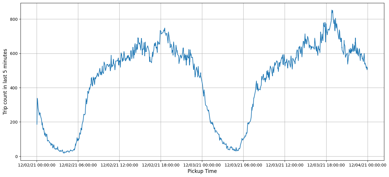
The taxi ride count reached its lowest point around 5:00 a.m., and peaked around 7:00 p.m. on a workday. Such is the rhythm of NYC.