# Copyright 2025 Google LLC
#
# Licensed under the Apache License, Version 2.0 (the "License");
# you may not use this file except in compliance with the License.
# You may obtain a copy of the License at
#
#     https://www.apache.org/licenses/LICENSE-2.0
#
# Unless required by applicable law or agreed to in writing, software
# distributed under the License is distributed on an "AS IS" BASIS,
# WITHOUT WARRANTIES OR CONDITIONS OF ANY KIND, either express or implied.
# See the License for the specific language governing permissions and
# limitations under the License.
BigFrames AI Forecast#
|
|
|
|
This Notebook introduces forecasting with GenAI Fundation Model with BigFrames AI.
Setup#
PROJECT = "bigframes-dev" # replace with your project

import bigframes.pandas as bpd
bpd.options.bigquery.project = PROJECT
bpd.options.display.progress_bar = None

# Optional, but recommended: partial ordering mode can accelerate executions and save costs.
bpd.options.bigquery.ordering_mode = "partial"
1. Create a BigFrames DataFrames from BigQuery public data.#
df = bpd.read_gbq("bigquery-public-data.san_francisco_bikeshare.bikeshare_trips")
df
| trip_id | duration_sec | start_date | start_station_name | start_station_id | end_date | end_station_name | end_station_id | bike_number | zip_code | ... | c_subscription_type | start_station_latitude | start_station_longitude | end_station_latitude | end_station_longitude | member_birth_year | member_gender | bike_share_for_all_trip | start_station_geom | end_station_geom | |
|---|---|---|---|---|---|---|---|---|---|---|---|---|---|---|---|---|---|---|---|---|---|
| 0 | 20171215164722144 | 501 | 2017-12-15 16:47:22+00:00 | 10th St at Fallon St | 201 | 2017-12-15 16:55:44+00:00 | 10th Ave at E 15th St | 222 | 144 | <NA> | ... | <NA> | 37.797673 | -122.262997 | 37.792714 | -122.24878 | 1984 | Male | <NA> | POINT (-122.263 37.79767) | POINT (-122.24878 37.79271) |
| 1 | 201708052346051585 | 712 | 2017-08-05 23:46:05+00:00 | 10th St at Fallon St | 201 | 2017-08-05 23:57:57+00:00 | 10th Ave at E 15th St | 222 | 1585 | <NA> | ... | <NA> | 37.797673 | -122.262997 | 37.792714 | -122.24878 | <NA> | <NA> | <NA> | POINT (-122.263 37.79767) | POINT (-122.24878 37.79271) |
| 2 | 201711111447202880 | 272 | 2017-11-11 14:47:20+00:00 | 12th St at 4th Ave | 233 | 2017-11-11 14:51:53+00:00 | 10th Ave at E 15th St | 222 | 2880 | <NA> | ... | <NA> | 37.795812 | -122.255555 | 37.792714 | -122.24878 | 1965 | Female | <NA> | POINT (-122.25555 37.79581) | POINT (-122.24878 37.79271) |
| 3 | 201804251726273755 | 757 | 2018-04-25 17:26:27+00:00 | 13th St at Franklin St | 338 | 2018-04-25 17:39:05+00:00 | 10th Ave at E 15th St | 222 | 3755 | <NA> | ... | <NA> | 37.803189 | -122.270579 | 37.792714 | -122.24878 | 1982 | Other | No | POINT (-122.27058 37.80319) | POINT (-122.24878 37.79271) |
| 4 | 20180408155601183 | 1105 | 2018-04-08 15:56:01+00:00 | 13th St at Franklin St | 338 | 2018-04-08 16:14:26+00:00 | 10th Ave at E 15th St | 222 | 183 | <NA> | ... | <NA> | 37.803189 | -122.270579 | 37.792714 | -122.24878 | 1987 | Female | No | POINT (-122.27058 37.80319) | POINT (-122.24878 37.79271) |
| 5 | 201804191648501560 | 857 | 2018-04-19 16:48:50+00:00 | 13th St at Franklin St | 338 | 2018-04-19 17:03:08+00:00 | 10th Ave at E 15th St | 222 | 1560 | <NA> | ... | <NA> | 37.803189 | -122.270579 | 37.792714 | -122.24878 | 1982 | Other | No | POINT (-122.27058 37.80319) | POINT (-122.24878 37.79271) |
| 6 | 20170810204454839 | 1256 | 2017-08-10 20:44:54+00:00 | 2nd Ave at E 18th St | 200 | 2017-08-10 21:05:50+00:00 | 10th Ave at E 15th St | 222 | 839 | <NA> | ... | <NA> | 37.800214 | -122.25381 | 37.792714 | -122.24878 | <NA> | <NA> | <NA> | POINT (-122.25381 37.80021) | POINT (-122.24878 37.79271) |
| 7 | 20171012204438666 | 630 | 2017-10-12 20:44:38+00:00 | 2nd Ave at E 18th St | 200 | 2017-10-12 20:55:09+00:00 | 10th Ave at E 15th St | 222 | 666 | <NA> | ... | <NA> | 37.800214 | -122.25381 | 37.792714 | -122.24878 | <NA> | <NA> | <NA> | POINT (-122.25381 37.80021) | POINT (-122.24878 37.79271) |
| 8 | 201711181823281960 | 353 | 2017-11-18 18:23:28+00:00 | 2nd Ave at E 18th St | 200 | 2017-11-18 18:29:22+00:00 | 10th Ave at E 15th St | 222 | 1960 | <NA> | ... | <NA> | 37.800214 | -122.25381 | 37.792714 | -122.24878 | 1988 | Male | <NA> | POINT (-122.25381 37.80021) | POINT (-122.24878 37.79271) |
| 9 | 20170806183917510 | 298 | 2017-08-06 18:39:17+00:00 | 2nd Ave at E 18th St | 200 | 2017-08-06 18:44:15+00:00 | 10th Ave at E 15th St | 222 | 510 | <NA> | ... | <NA> | 37.800214 | -122.25381 | 37.792714 | -122.24878 | 1969 | Male | <NA> | POINT (-122.25381 37.80021) | POINT (-122.24878 37.79271) |
10 rows × 21 columns
2. Preprocess Data#
Only take the start_date after 2018 and the “Subscriber” category as input. start_date are truncated to each hour.
df = df[df["start_date"] >= "2018-01-01"]
df = df[df["subscriber_type"] == "Subscriber"]
df["trip_hour"] = df["start_date"].dt.floor("h")
df = df[["trip_hour", "trip_id"]]
Group and count each hour’s num of trips.
df_grouped = df.groupby("trip_hour").count()
df_grouped = df_grouped.reset_index().rename(columns={"trip_id": "num_trips"})
df_grouped
| trip_hour | num_trips | |
|---|---|---|
| 0 | 2018-01-01 00:00:00+00:00 | 20 |
| 1 | 2018-01-01 01:00:00+00:00 | 25 |
| 2 | 2018-01-01 02:00:00+00:00 | 13 |
| 3 | 2018-01-01 03:00:00+00:00 | 11 |
| 4 | 2018-01-01 05:00:00+00:00 | 4 |
| 5 | 2018-01-01 06:00:00+00:00 | 8 |
| 6 | 2018-01-01 07:00:00+00:00 | 8 |
| 7 | 2018-01-01 08:00:00+00:00 | 20 |
| 8 | 2018-01-01 09:00:00+00:00 | 30 |
| 9 | 2018-01-01 10:00:00+00:00 | 41 |
10 rows × 2 columns
3. Make forecastings for next 1 week with DataFrames.ai.forecast API#
import bigframes.bigquery as bbq

# Using all the data except the last week (2842-168) for training. And predict the last week (168).
result = bbq.ai.forecast(df_grouped.head(2842-168), timestamp_col="trip_hour", data_col="num_trips", horizon=168)
result
| forecast_timestamp | forecast_value | confidence_level | prediction_interval_lower_bound | prediction_interval_upper_bound | ai_forecast_status | |
|---|---|---|---|---|---|---|
| 0 | 2018-04-24 12:00:00+00:00 | 147.023743 | 0.95 | 98.736624 | 195.310862 | |
| 1 | 2018-04-25 00:00:00+00:00 | 6.955032 | 0.95 | -6.094232 | 20.004297 | |
| 2 | 2018-04-26 05:00:00+00:00 | -37.196533 | 0.95 | -88.759566 | 14.366499 | |
| 3 | 2018-04-26 14:00:00+00:00 | 115.635132 | 0.95 | 30.120832 | 201.149432 | |
| 4 | 2018-04-27 02:00:00+00:00 | 2.516006 | 0.95 | -69.095591 | 74.127604 | |
| 5 | 2018-04-29 03:00:00+00:00 | 22.503326 | 0.95 | -38.714378 | 83.721031 | |
| 6 | 2018-04-24 04:00:00+00:00 | -12.259079 | 0.95 | -45.377262 | 20.859104 | |
| 7 | 2018-04-24 14:00:00+00:00 | 126.519211 | 0.95 | 96.837778 | 156.200644 | |
| 8 | 2018-04-26 11:00:00+00:00 | 120.90567 | 0.95 | 35.781735 | 206.029606 | |
| 9 | 2018-04-27 13:00:00+00:00 | 162.023026 | 0.95 | 103.946307 | 220.099744 |
10 rows × 6 columns
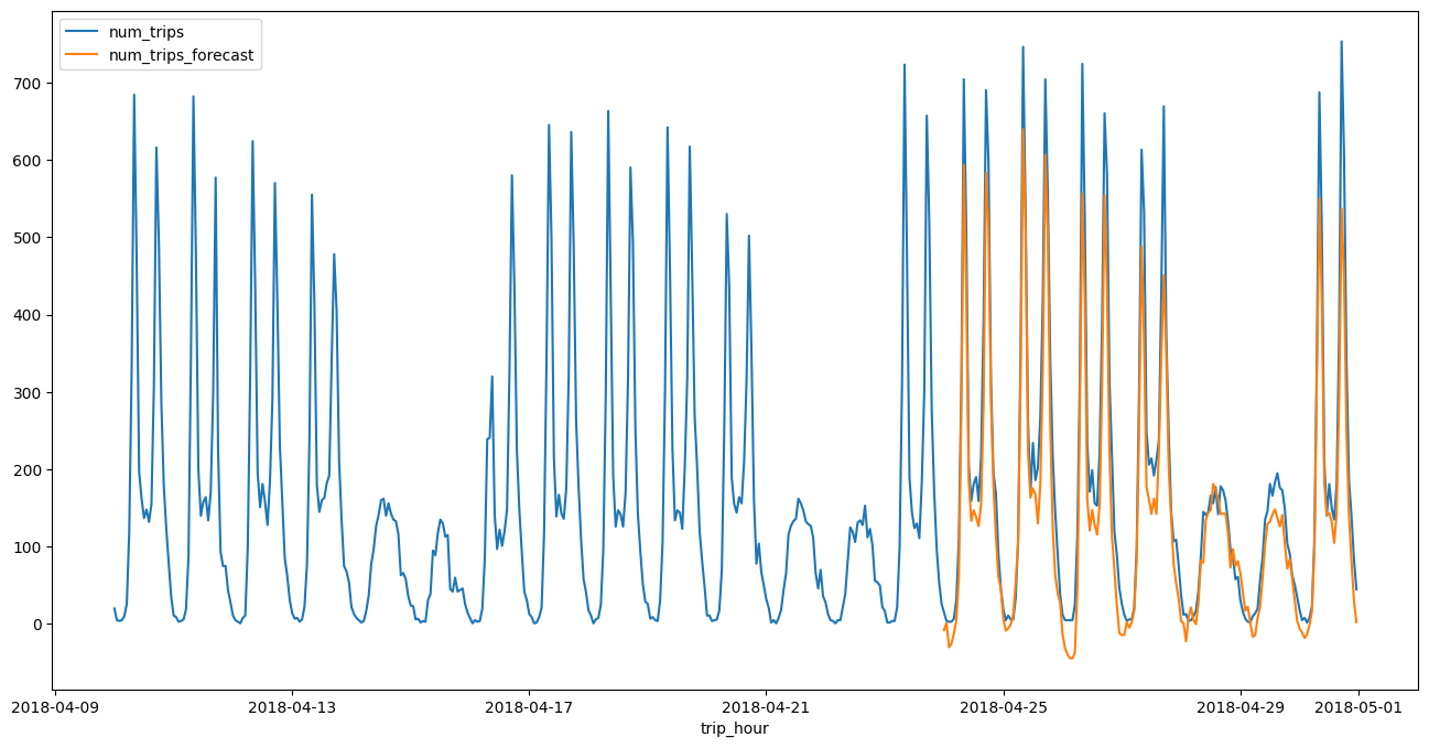
4. Process the raw result and draw a line plot along with the training data#
result = result.sort_values("forecast_timestamp")
result = result[["forecast_timestamp", "forecast_value"]]
result = result.rename(columns={"forecast_timestamp": "trip_hour", "forecast_value": "num_trips_forecast"})
df_all = bpd.concat([df_grouped, result])
df_all = df_all.tail(672) # 4 weeks
Plot a line chart and compare with the actual result.
df_all = df_all.set_index("trip_hour")
df_all.plot.line(figsize=(16, 8))
<Axes: xlabel='trip_hour'>